github:
https://github.com/pandalabme/d2l/tree/main/exercises
import sys
import torch.nn as nn
import torch
import warnings
sys.path.append('/home/jovyan/work/d2l_solutions/notebooks/exercises/d2l_utils/')
import d2l
from torchsummary import summary
warnings.filterwarnings("ignore")


def stat_params(net, params):
    for idx, module in enumerate(net):
        if type(module) not in (nn.Linear,nn.Conv2d):
            continue
        num = sum(p.numel() for p in module.parameters())
        if type(module) == nn.Conv2d:
            params['conv'] += num
        else:
            params['lr'] += num

def stat_comp(net, params, x):
    for idx, module in enumerate(net):
        c_i = x.shape[1]
        x = module(x)
        if type(module) == nn.Conv2d:
            k = [p.shape for p in module.parameters()]
            c_o,h_o,w_o = x.shape[1], x.shape[2], x.shape[3]
            params['conv'] += c_i*c_o*h_o*w_o*k[0][-1]*k[0][-2]
        if type(module) == nn.Linear:
            params['lr'] += sum(p.numel() for p in module.parameters())
    return x


def vgg_block(num_convs, out_channels):
    layers = []
    for _ in range(num_convs):
        layers.append(nn.LazyConv2d(out_channels, kernel_size=3, padding=1))
        layers.append(nn.ReLU())
    layers.append(nn.MaxPool2d(kernel_size=2, stride=2))
    return nn.Sequential(*layers)

class VGG(d2l.Classifier):
    def __init__(self, arch, lr=0.1, num_classes=10):
        super().__init__()
        self.save_hyperparameters()
        conv_blks = []
        for (num_convs, out_channels) in arch:
            conv_blks.append(vgg_block(num_convs, out_channels))
        self.net = nn.Sequential(*conv_blks, nn.Flatten(),
                                 nn.LazyLinear(4096), nn.ReLU(), nn.Dropout(0.5),
                                 nn.LazyLinear(4096), nn.ReLU(), nn.Dropout(0.5),
                                 nn.LazyLinear(num_classes))
        self.net.apply(d2l.init_cnn)
1. Compared with AlexNet, VGG is much slower in terms of computation, and it also needs more GPU memory.
1.1 Compare the number of parameters needed for AlexNet and VGG.
| vgg | alexnet | vgg/alexnet | |
|---|---|---|---|
| conv | 9220480 | 3747200 | 2.46 |
| lr | 119586826 | 43040778 | 2.77 |
arch=((1, 64), (1, 128), (2, 256), (2, 512), (2, 512))
vgg = VGG(arch=arch)
X = torch.randn(1,3, 224, 224)
_ = vgg(X)
params = {'conv':0, 'lr':0}
for idx, module in enumerate(vgg.net):
    if type(module) == nn.Sequential:
        stat_params(module,params)
    if type(module) == nn.Linear:
        num = sum(p.numel() for p in module.parameters())
        params['lr'] += num
summary(vgg, (3, 224, 224))
params
----------------------------------------------------------------
        Layer (type)               Output Shape         Param #
================================================================
            Conv2d-1         [-1, 64, 224, 224]           1,792
              ReLU-2         [-1, 64, 224, 224]               0
         MaxPool2d-3         [-1, 64, 112, 112]               0
            Conv2d-4        [-1, 128, 112, 112]          73,856
              ReLU-5        [-1, 128, 112, 112]               0
         MaxPool2d-6          [-1, 128, 56, 56]               0
            Conv2d-7          [-1, 256, 56, 56]         295,168
              ReLU-8          [-1, 256, 56, 56]               0
            Conv2d-9          [-1, 256, 56, 56]         590,080
             ReLU-10          [-1, 256, 56, 56]               0
        MaxPool2d-11          [-1, 256, 28, 28]               0
           Conv2d-12          [-1, 512, 28, 28]       1,180,160
             ReLU-13          [-1, 512, 28, 28]               0
           Conv2d-14          [-1, 512, 28, 28]       2,359,808
             ReLU-15          [-1, 512, 28, 28]               0
        MaxPool2d-16          [-1, 512, 14, 14]               0
           Conv2d-17          [-1, 512, 14, 14]       2,359,808
             ReLU-18          [-1, 512, 14, 14]               0
           Conv2d-19          [-1, 512, 14, 14]       2,359,808
             ReLU-20          [-1, 512, 14, 14]               0
        MaxPool2d-21            [-1, 512, 7, 7]               0
          Flatten-22                [-1, 25088]               0
           Linear-23                 [-1, 4096]     102,764,544
             ReLU-24                 [-1, 4096]               0
          Dropout-25                 [-1, 4096]               0
           Linear-26                 [-1, 4096]      16,781,312
             ReLU-27                 [-1, 4096]               0
          Dropout-28                 [-1, 4096]               0
           Linear-29                   [-1, 10]          40,970
================================================================
Total params: 128,807,306
Trainable params: 128,807,306
Non-trainable params: 0
----------------------------------------------------------------
Input size (MB): 0.57
Forward/backward pass size (MB): 125.37
Params size (MB): 491.36
Estimated Total Size (MB): 617.30
----------------------------------------------------------------


{'conv': 9220480, 'lr': 119586826}
1.2 Compare the number of floating point operations used in the convolutional layers and in the fully connected layers.
| vgg | alexnet | vgg/alexnet | |
|---|---|---|---|
| conv | 7485456384 | 962858112 | 7.77 |
| lr | 119586826 | 43040778 | 2.77 |
x = torch.randn(1,3, 224, 224)
params = {'conv':0, 'lr':0}
for idx, module in enumerate(vgg.net):
    if type(module) == nn.Sequential:
        x = stat_comp(module, params, x)
    if type(module) == nn.Linear:
        params['lr'] += sum(p.numel() for p in module.parameters())
params
{'conv': 7485456384, 'lr': 119586826}
1.3 How could you reduce the computational cost created by the fully connected layers?
Reducing the computational cost created by fully connected layers can help improve the efficiency of neural networks while maintaining or even enhancing their performance. Here are several strategies to achieve this:
-
Global Average Pooling (GAP):
Instead of using fully connected layers at the end of the network, apply global average pooling. This operation computes the average of each feature map and produces a single value for each channel. GAP reduces the number of parameters and computations significantly while retaining important spatial information. -
Replace with Convolutional Layers:
Convert fully connected layers into convolutional layers with kernel size 1x1. This allows for weight sharing across spatial locations and reduces the number of parameters. Transition from fully connected layers to 1x1 convolutions can often be done without sacrificing performance. -
Network Pruning:
Apply network pruning techniques to identify and remove unnecessary connections, neurons, or filters in the fully connected layers. Pruning reduces the number of parameters and computations while maintaining accuracy. -
Low-Rank Approximations:
Approximate fully connected weight matrices with low-rank matrices using techniques like Singular Value Decomposition (SVD). This reduces the number of parameters and speeds up computations. -
Dimension Reduction Techniques:
Apply dimensionality reduction techniques such as Principal Component Analysis (PCA) to reduce the input dimensionality of fully connected layers. This can reduce the number of parameters and computations required. -
Depthwise Separable Convolutions:
Replace fully connected layers with depthwise separable convolutions. These convolutions separate spatial and channel-wise filtering, reducing the number of parameters and computations. -
Quantization:
Quantize fully connected layers to lower precision (e.g., 8-bit) to reduce memory usage and computation. Techniques like quantization-aware training can help minimize the impact on accuracy. -
Knowledge Distillation:
Use knowledge distillation to train a smaller student network to mimic the behavior of a larger teacher network. This can help maintain performance while reducing the computational cost. -
Model Compression:
Apply model compression techniques like Huffman coding, weight sharing, or tensor factorization to reduce the size and computational complexity of fully connected layers. -
Hybrid Architectures:
Design hybrid architectures that combine convolutional and fully connected layers. Use fully connected layers only in specific parts of the network where they are essential.
It’s important to note that the effectiveness of these strategies can vary based on the specific architecture, dataset, and task. Experimentation and tuning are necessary to find the optimal trade-off between computational cost reduction and performance.
2. When displaying the dimensions associated with the various layers of the network, we only see the information associated with eight blocks (plus some auxiliary transforms), even though the network has 11 layers. Where did the remaining three layers go?
The convolutional block is looked as one layer in network, and the latter three convolutional blocks in vgg contain two convolutional layers each, these are the remaining three layers.
vgg
VGG(
  (net): Sequential(
    (0): Sequential(
      (0): Conv2d(3, 64, kernel_size=(3, 3), stride=(1, 1), padding=(1, 1))
      (1): ReLU()
      (2): MaxPool2d(kernel_size=2, stride=2, padding=0, dilation=1, ceil_mode=False)
    )
    (1): Sequential(
      (0): Conv2d(64, 128, kernel_size=(3, 3), stride=(1, 1), padding=(1, 1))
      (1): ReLU()
      (2): MaxPool2d(kernel_size=2, stride=2, padding=0, dilation=1, ceil_mode=False)
    )
    (2): Sequential(
      (0): Conv2d(128, 256, kernel_size=(3, 3), stride=(1, 1), padding=(1, 1))
      (1): ReLU()
      (2): Conv2d(256, 256, kernel_size=(3, 3), stride=(1, 1), padding=(1, 1))
      (3): ReLU()
      (4): MaxPool2d(kernel_size=2, stride=2, padding=0, dilation=1, ceil_mode=False)
    )
    (3): Sequential(
      (0): Conv2d(256, 512, kernel_size=(3, 3), stride=(1, 1), padding=(1, 1))
      (1): ReLU()
      (2): Conv2d(512, 512, kernel_size=(3, 3), stride=(1, 1), padding=(1, 1))
      (3): ReLU()
      (4): MaxPool2d(kernel_size=2, stride=2, padding=0, dilation=1, ceil_mode=False)
    )
    (4): Sequential(
      (0): Conv2d(512, 512, kernel_size=(3, 3), stride=(1, 1), padding=(1, 1))
      (1): ReLU()
      (2): Conv2d(512, 512, kernel_size=(3, 3), stride=(1, 1), padding=(1, 1))
      (3): ReLU()
      (4): MaxPool2d(kernel_size=2, stride=2, padding=0, dilation=1, ceil_mode=False)
    )
    (5): Flatten(start_dim=1, end_dim=-1)
    (6): Linear(in_features=25088, out_features=4096, bias=True)
    (7): ReLU()
    (8): Dropout(p=0.5, inplace=False)
    (9): Linear(in_features=4096, out_features=4096, bias=True)
    (10): ReLU()
    (11): Dropout(p=0.5, inplace=False)
    (12): Linear(in_features=4096, out_features=10, bias=True)
  )
)
3. Use Table 1 in the VGG paper (Simonyan and Zisserman, 2014) to construct other common models, such as VGG-16 or VGG-19.
arch16=((2, 64), (2, 128), (3, 256), (32, 512), (3, 512))
vgg16 = VGG(arch=arch16)
vgg16
VGG(
  (net): Sequential(
    (0): Sequential(
      (0): LazyConv2d(0, 64, kernel_size=(3, 3), stride=(1, 1), padding=(1, 1))
      (1): ReLU()
      (2): LazyConv2d(0, 64, kernel_size=(3, 3), stride=(1, 1), padding=(1, 1))
      (3): ReLU()
      (4): MaxPool2d(kernel_size=2, stride=2, padding=0, dilation=1, ceil_mode=False)
    )
    (1): Sequential(
      (0): LazyConv2d(0, 128, kernel_size=(3, 3), stride=(1, 1), padding=(1, 1))
      (1): ReLU()
      (2): LazyConv2d(0, 128, kernel_size=(3, 3), stride=(1, 1), padding=(1, 1))
      (3): ReLU()
      (4): MaxPool2d(kernel_size=2, stride=2, padding=0, dilation=1, ceil_mode=False)
    )
    (2): Sequential(
      (0): LazyConv2d(0, 256, kernel_size=(3, 3), stride=(1, 1), padding=(1, 1))
      (1): ReLU()
      (2): LazyConv2d(0, 256, kernel_size=(3, 3), stride=(1, 1), padding=(1, 1))
      (3): ReLU()
      (4): LazyConv2d(0, 256, kernel_size=(3, 3), stride=(1, 1), padding=(1, 1))
      (5): ReLU()
      (6): MaxPool2d(kernel_size=2, stride=2, padding=0, dilation=1, ceil_mode=False)
    )
    (3): Sequential(
      (0): LazyConv2d(0, 512, kernel_size=(3, 3), stride=(1, 1), padding=(1, 1))
      (1): ReLU()
      (2): LazyConv2d(0, 512, kernel_size=(3, 3), stride=(1, 1), padding=(1, 1))
      (3): ReLU()
      (4): LazyConv2d(0, 512, kernel_size=(3, 3), stride=(1, 1), padding=(1, 1))
      (5): ReLU()
      (6): LazyConv2d(0, 512, kernel_size=(3, 3), stride=(1, 1), padding=(1, 1))
      (7): ReLU()
      (8): LazyConv2d(0, 512, kernel_size=(3, 3), stride=(1, 1), padding=(1, 1))
      (9): ReLU()
      (10): LazyConv2d(0, 512, kernel_size=(3, 3), stride=(1, 1), padding=(1, 1))
      (11): ReLU()
      (12): LazyConv2d(0, 512, kernel_size=(3, 3), stride=(1, 1), padding=(1, 1))
      (13): ReLU()
      (14): LazyConv2d(0, 512, kernel_size=(3, 3), stride=(1, 1), padding=(1, 1))
      (15): ReLU()
      (16): LazyConv2d(0, 512, kernel_size=(3, 3), stride=(1, 1), padding=(1, 1))
      (17): ReLU()
      (18): LazyConv2d(0, 512, kernel_size=(3, 3), stride=(1, 1), padding=(1, 1))
      (19): ReLU()
      (20): LazyConv2d(0, 512, kernel_size=(3, 3), stride=(1, 1), padding=(1, 1))
      (21): ReLU()
      (22): LazyConv2d(0, 512, kernel_size=(3, 3), stride=(1, 1), padding=(1, 1))
      (23): ReLU()
      (24): LazyConv2d(0, 512, kernel_size=(3, 3), stride=(1, 1), padding=(1, 1))
      (25): ReLU()
      (26): LazyConv2d(0, 512, kernel_size=(3, 3), stride=(1, 1), padding=(1, 1))
      (27): ReLU()
      (28): LazyConv2d(0, 512, kernel_size=(3, 3), stride=(1, 1), padding=(1, 1))
      (29): ReLU()
      (30): LazyConv2d(0, 512, kernel_size=(3, 3), stride=(1, 1), padding=(1, 1))
      (31): ReLU()
      (32): LazyConv2d(0, 512, kernel_size=(3, 3), stride=(1, 1), padding=(1, 1))
      (33): ReLU()
      (34): LazyConv2d(0, 512, kernel_size=(3, 3), stride=(1, 1), padding=(1, 1))
      (35): ReLU()
      (36): LazyConv2d(0, 512, kernel_size=(3, 3), stride=(1, 1), padding=(1, 1))
      (37): ReLU()
      (38): LazyConv2d(0, 512, kernel_size=(3, 3), stride=(1, 1), padding=(1, 1))
      (39): ReLU()
      (40): LazyConv2d(0, 512, kernel_size=(3, 3), stride=(1, 1), padding=(1, 1))
      (41): ReLU()
      (42): LazyConv2d(0, 512, kernel_size=(3, 3), stride=(1, 1), padding=(1, 1))
      (43): ReLU()
      (44): LazyConv2d(0, 512, kernel_size=(3, 3), stride=(1, 1), padding=(1, 1))
      (45): ReLU()
      (46): LazyConv2d(0, 512, kernel_size=(3, 3), stride=(1, 1), padding=(1, 1))
      (47): ReLU()
      (48): LazyConv2d(0, 512, kernel_size=(3, 3), stride=(1, 1), padding=(1, 1))
      (49): ReLU()
      (50): LazyConv2d(0, 512, kernel_size=(3, 3), stride=(1, 1), padding=(1, 1))
      (51): ReLU()
      (52): LazyConv2d(0, 512, kernel_size=(3, 3), stride=(1, 1), padding=(1, 1))
      (53): ReLU()
      (54): LazyConv2d(0, 512, kernel_size=(3, 3), stride=(1, 1), padding=(1, 1))
      (55): ReLU()
      (56): LazyConv2d(0, 512, kernel_size=(3, 3), stride=(1, 1), padding=(1, 1))
      (57): ReLU()
      (58): LazyConv2d(0, 512, kernel_size=(3, 3), stride=(1, 1), padding=(1, 1))
      (59): ReLU()
      (60): LazyConv2d(0, 512, kernel_size=(3, 3), stride=(1, 1), padding=(1, 1))
      (61): ReLU()
      (62): LazyConv2d(0, 512, kernel_size=(3, 3), stride=(1, 1), padding=(1, 1))
      (63): ReLU()
      (64): MaxPool2d(kernel_size=2, stride=2, padding=0, dilation=1, ceil_mode=False)
    )
    (4): Sequential(
      (0): LazyConv2d(0, 512, kernel_size=(3, 3), stride=(1, 1), padding=(1, 1))
      (1): ReLU()
      (2): LazyConv2d(0, 512, kernel_size=(3, 3), stride=(1, 1), padding=(1, 1))
      (3): ReLU()
      (4): LazyConv2d(0, 512, kernel_size=(3, 3), stride=(1, 1), padding=(1, 1))
      (5): ReLU()
      (6): MaxPool2d(kernel_size=2, stride=2, padding=0, dilation=1, ceil_mode=False)
    )
    (5): Flatten(start_dim=1, end_dim=-1)
    (6): LazyLinear(in_features=0, out_features=4096, bias=True)
    (7): ReLU()
    (8): Dropout(p=0.5, inplace=False)
    (9): LazyLinear(in_features=0, out_features=4096, bias=True)
    (10): ReLU()
    (11): Dropout(p=0.5, inplace=False)
    (12): LazyLinear(in_features=0, out_features=10, bias=True)
  )
)
arch19=((2, 64), (2, 128), (3, 256), (32, 512), (3, 512))
vgg19 = VGG(arch=arch16)
vgg16
4. Upsampling the resolution in Fashion-MNIST eight-fold from 28\times28 to 224\times224 dimensions is very wasteful. Try modifying the network architecture and resolution conversion, e.g., to 56 or to 84 dimensions for its input instead. Can you do so without reducing the accuracy of the network? Consult the VGG paper (Simonyan and Zisserman, 2014) for ideas on adding more nonlinearities prior to downsampling.
model = VGG(arch=((3, 128), (3, 256)), lr=0.01)
trainer = d2l.Trainer(max_epochs=10, num_gpus=1)
data = d2l.FashionMNIST(batch_size=128, resize=(28, 28))
trainer.fit(model, data)
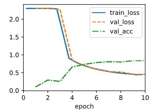
acc: 0.84