github:
https://github.com/pandalabme/d2l/tree/main/exercises

1. Change the number of hidden units num_hiddens and plot how its number affects the accuracy of the model. What is the best value of this hyperparameter?

As the number of hidden units grows, accuracy of the model increases first and goes down after 4096, so 4096 might be the best value of this hyperparameter

def stat_acc(num_hiddens):
    model = MLP(num_outputs=10, num_hiddens=num_hiddens, lr=0.1)
    trainer = d2l.Trainer(max_epochs=10, plot_flag=False)
    trainer.fit(model, data)
    y_hat = model(data.val.data.type(torch.float32))
    return model.accuracy(y_hat,data.val.targets).item()

hiddens = d2l.gen_logrithm_nums(initial_value = 64, growth_factor = 2, num_elements = 8)
accs = []
for num_hiddens in tqdm(hiddens):
    accs.append(stat_acc(num_hiddens))

100%|██████████| 8/8 [23:02<00:00, 172.78s/it]

d2l.plot(hiddens,accs,'num_hiddens','acc')

2. Try adding a hidden layer to see how it affects the results.

As we add a hidden layer, the accuracy improves.

class MulMLP(d2l.Classifier):
    def __init__(self, num_outputs, num_hiddens, lr):
        super().__init__()
        self.save_hyperparameters()
        layers = [nn.Flatten()]
        for num in num_hiddens:
            layers.append(nn.LazyLinear(num))
            layers.append(nn.ReLU())
        layers.append(nn.LazyLinear(num_outputs))
        self.net = nn.Sequential(*layers)

model = MulMLP(num_outputs=10, num_hiddens=[256,128], lr=0.1)
trainer = d2l.Trainer(max_epochs=10, plot_flag=True)
trainer.fit(model, data)
y_hat = model(data.val.data.type(torch.float32)) 
print(f'acc: {model.accuracy(y_hat,data.val.targets).item():.2f}')

acc: 0.79

3. Why is it a bad idea to insert a hidden layer with a single neuron? What could go wrong?

Inserting a hidden layer with a single neuron in a neural network can lead to several issues and limitations. This configuration is often referred to as a “bottleneck layer” or “degenerate layer.” While it’s not inherently incorrect, it can have negative consequences for the network’s performance, training dynamics, and capacity to learn complex patterns. Here are some of the problems that can arise:

1. Loss of Expressiveness: A single neuron in a hidden layer severely limits the expressive power of the network. Neural networks derive their power from their ability to model complex nonlinear relationships through multiple layers and neurons. A single neuron cannot capture complex relationships, leading to a lack of representational capacity.

2. Limited Feature Learning: Neural networks typically learn useful features in hidden layers through a hierarchy of representations. A single hidden neuron lacks the capacity to learn diverse and meaningful features, which can hinder the network’s ability to generalize from the data.

3. High Bias: A single neuron can easily become biased towards capturing a specific pattern or representation, leading to poor generalization to new data. The network may overfit to the training data and fail to capture the underlying patterns.

4. Vanishing Gradients: With just one neuron in the hidden layer, the gradients that flow backward during training can become extremely small or even vanish. This makes weight updates difficult, leading to slow convergence or no convergence at all.

5. Lack of Nonlinearity: Hidden layers with multiple neurons allow the network to capture nonlinear relationships. A single neuron can only provide linear transformations, limiting the network’s ability to capture complex, nonlinear data distributions.

6. No Hierarchical Learning: The power of deep learning comes from learning hierarchical features at different levels of abstraction. A single neuron doesn’t allow for the creation of such hierarchical representations.

7. Poor Capacity to Approximate Functions: Neural networks with multiple neurons and layers can approximate a wide range of functions. A single-neuron hidden layer lacks the capacity to approximate complex functions and patterns.

8. Difficulty in Optimization: Optimizing the weights of a single neuron can be challenging. The optimization landscape might have sharp and narrow minima, making it hard for gradient-based optimization methods to find suitable weights.

9. Network Robustness: A single neuron layer can make the network more vulnerable to adversarial attacks and noise in the data.

In summary, adding a hidden layer with a single neuron can lead to a severely underpowered neural network that struggles to capture complex relationships in data, suffers from vanishing gradients, and lacks the capacity for hierarchical feature learning. It’s crucial to design networks with an appropriate number of neurons and layers to ensure the network’s capacity to learn and generalize from the data effectively.

4. How does changing the learning rate alter your results? With all other parameters fixed, which learning rate gives you the best results? How does this relate to the number of epochs?

• As learning rate improves, accuracy of the model increases first and goes down after 0.01, so 0.01 might be the best value of this hyperparameter
• As the number of epochs increases, train accuracy goes up, while test accuracy improves first and decrease latter.

def stat_lr(lr):
    model = MLP(num_outputs=10, num_hiddens=256, lr=lr)
    trainer = d2l.Trainer(max_epochs=10, plot_flag=True)
    trainer.fit(model, data)
    y_hat = model(data.val.data.type(torch.float32))
    return model.accuracy(y_hat,data.val.targets).item()

lrs = [0.001, 0.01, 0.03, 0.1, 0.3, 1]
accs = []
accs.append(stat_lr(lrs[0]))

accs.append(stat_lr(lrs[1]))

accs.append(stat_lr(lrs[2]))

accs.append(stat_lr(lrs[3]))

accs.append(stat_lr(lrs[4]))

accs.append(stat_lr(lrs[5]))

d2l.plot(lrs,accs[-len(lrs):],'lr','acc')

model = MLP(num_outputs=10, num_hiddens=256, lr=0.1)
trainer = d2l.Trainer(max_epochs=10, plot_flag=False)
trainer.fit(model, data)

5. Let’s optimize over all hyperparameters jointly, i.e., learning rate, number of epochs, number of hidden layers, and number of hidden units per layer.

• What is the best result you can get by optimizing over all of them?
• Why it is much more challenging to deal with multiple hyperparameters?
• Describe an efficient strategy for optimizing over multiple parameters jointly.

Optimizing over multiple hyperparameters jointly is a complex task, often referred to as hyperparameter tuning or hyperparameter optimization. Let’s address your questions one by one:

1. Best Result by Jointly Optimizing All Hyperparameters:

The best result you can achieve by optimizing all hyperparameters jointly depends on the problem, dataset, and the interaction between hyperparameters. There’s no universal answer as it’s highly specific to the task. In some cases, a carefully optimized model might significantly outperform a default or randomly chosen hyperparameter configuration, leading to improved accuracy, convergence speed, and generalization. However, the absolute “best” result is challenging to determine due to the complexity of the optimization landscape.

2. Challenges of Dealing with Multiple Hyperparameters:

Dealing with multiple hyperparameters is more challenging due to the following reasons:

• Curse of Dimensionality: As you increase the number of hyperparameters, the search space grows exponentially, making it harder to explore efficiently.

• Interaction Effects: Hyperparameters can interact with each other in complex ways, affecting the overall behavior of the model. For example, the learning rate might impact the convergence behavior differently depending on the number of hidden layers or units.

• Noisy or Uncertain Feedback: The evaluation of a specific hyperparameter configuration might be noisy due to factors like random initialization, data variability, or runtime fluctuations.

• Limited Resources: Limited computational resources and time make exhaustive search impractical, requiring smarter search strategies.

3. Efficient Strategy for Joint Optimization:

Efficiently optimizing over multiple parameters requires a systematic approach. One commonly used strategy is Bayesian Optimization, which combines probability models and an acquisition function to guide the search towards promising regions of the hyperparameter space. Here’s a general outline of the process:

1. Define a Search Space: Define ranges or distributions for each hyperparameter that you want to optimize.

2. Select an Acquisition Function: Choose an acquisition function (e.g., Expected Improvement, Upper Confidence Bound) that guides the search based on the uncertainty and predicted performance of different hyperparameter configurations.

3. Build a Surrogate Model: Create a probabilistic model that approximates the unknown relationship between hyperparameters and performance. Gaussian Process Regression is often used for this purpose.

4. Iterative Search: Start with an initial set of hyperparameters and evaluate the model’s performance. Use the surrogate model and acquisition function to select the next hyperparameters to evaluate. Repeat this process iteratively, updating the surrogate model based on new evaluations.

5. Convergence Criteria: Stop the optimization process when a predefined number of iterations is reached or when the acquisition function suggests that exploration is unlikely to lead to further improvements.

Bayesian Optimization can help navigate the complex optimization landscape efficiently by focusing on promising regions and adapting the search based on the outcomes of past evaluations.

Remember that hyperparameter tuning is an iterative process, and the optimal configuration might depend on experimentation, domain knowledge, and the specifics of your problem. It’s important to balance the exploration of hyperparameter space with the available computational resources and time

6. Compare the speed of the framework and the from-scratch implementation for a challenging problem. How does it change with the complexity of the network?

Comparing the speed of a deep learning framework like PyTorch with a from-scratch implementation for a challenging problem can be insightful, as it provides an understanding of the performance benefits and trade-offs of each approach. The speed comparison can be affected by various factors, including the problem complexity, network architecture, data size, and hardware resources.

Here’s how the speed comparison might change with the complexity of the network:

1. Simple Network:
   For a relatively simple network architecture with a small number of layers and parameters, the speed difference between a framework and a from-scratch implementation might not be as significant. The overhead introduced by the framework’s abstractions and optimizations could be more noticeable relative to the problem’s complexity.

2. Moderate Complexity:
   As the network complexity increases, with more layers, units, and parameters, the deep learning framework’s optimizations can become more valuable. Frameworks often leverage GPU acceleration, optimized tensor operations, and parallelism, resulting in significant speed improvements compared to a purely from-scratch implementation.

3. Complex Network:
   In the case of complex architectures like deep convolutional networks or large-scale recurrent networks, the gap in speed between the framework and from-scratch implementation can be substantial. The deep learning framework’s low-level optimizations, automatic differentiation, and GPU acceleration can provide a significant advantage, enabling faster training and convergence.

4. Batch Processing:
   The deep learning framework’s ability to efficiently process mini-batches of data further contributes to its speed advantage. Frameworks can take advantage of vectorized operations and parallelism to process multiple data points simultaneously, leading to faster updates of model parameters.

5. Hardware Utilization:
   The use of specialized hardware, such as GPUs or TPUs, can greatly accelerate training in a framework. These hardware devices are optimized for tensor operations and can significantly outperform CPUs in terms of both computation and memory bandwidth.

6. Custom Implementation Control:
   While a from-scratch implementation might provide more control over every aspect of the process, including initialization methods, optimization algorithms, and convergence criteria, it usually comes at the cost of development time and potentially slower execution.

In summary, deep learning frameworks like PyTorch are designed to optimize training efficiency and provide a balance between performance and flexibility. They leverage hardware acceleration, automatic differentiation, and optimizations to significantly speed up the training process, especially for complex network architectures. A from-scratch implementation, on the other hand, might offer more customization but can be significantly slower, especially for challenging problems involving complex networks.

class MulMLPScratch(d2l.Classifier):
    def __init__(self, num_inputs, num_outputs, num_hiddens, lr, sigma=0.01):
        super().__init__()
        self.save_hyperparameters()
        bef = num_inputs
        self.W = []
        self.b = []
        for num_hidden in num_hiddens:
            self.W.append(nn.Parameter(torch.randn(bef, num_hidden)*sigma))
            self.b.append(nn.Parameter(torch.zeros(num_hidden)))
            bef = num_hidden
        self.W.append(nn.Parameter(torch.randn(bef, num_outputs)*sigma))
        self.b.append(nn.Parameter(torch.zeros(num_outputs)))
        
        
    def forward(self, X):
        H = X.reshape(-1, self.num_inputs)
        for i in range(len(self.W)-1):
            H = relu(torch.matmul(H, self.W[i]) + self.b[i])
        return torch.matmul(H, self.W[-1]) + self.b[-1]
    
    def configure_optimizers(self):
        return d2l.SGD([*self.W, *self.b], self.lr)

def stat_time(model, data):
    t0 = time.time()
    trainer = d2l.Trainer(max_epochs=10, plot_flag=False)
    trainer.fit(model, data)
    return time.time() - t0

num_hiddens=[256,128,64,32,16]
ts = []
ts_strach = []
for i in tqdm(range(1,len(num_hiddens)+1)):
    model = MulMLP(num_outputs=10, num_hiddens=num_hiddens[:i], lr=0.1)
    model_scratch = MulMLPScratch(num_inputs=784, num_outputs=10, num_hiddens=num_hiddens[:i], lr=0.1)
    ts_strach.append(stat_time(model_scratch, data))
    ts.append(stat_time(model, data))

100%|██████████| 5/5 [23:18<00:00, 279.79s/it]

d2l.plot(list(range(1,len(num_hiddens)+1)),[ts,ts_strach],legend=['framework','scratch'])

7. Measure the speed of tensor–matrix multiplications for well-aligned and misaligned matrices. For instance, test for matrices with dimension 1024, 1025, 1026, 1028, and 1032.

• How does this change between GPUs and CPUs?
• Determine the memory bus width of your CPU and GPU.
  To measure the speed of tensor-matrix multiplications for well-aligned and misaligned matrices, and to analyze the differences between GPUs and CPUs, you can use PyTorch and the torch library. Additionally, determining the memory bus width requires information about the specific GPU and CPU models you’re using.

Here’s how you can perform the measurements and gather memory bus width information:

import torch
import time

# List of matrix dimensions to test
matrix_dimensions = [1024, 1025, 1026, 1028, 1032]

# Perform tensor-matrix multiplication and measure execution time
def measure_multiplication_speed(matrix_dim, device):
    torch.manual_seed(42)  # Set seed for reproducibility
    matrix = torch.randn(matrix_dim, matrix_dim).to(device)
    vector = torch.randn(matrix_dim, 1).to(device)
    
    start_time = time.time()
    result = torch.matmul(matrix, vector)
    end_time = time.time()
    
    execution_time = end_time - start_time
    return execution_time

# Test on CPU
print("CPU:")
for dim in matrix_dimensions:
    cpu_time = measure_multiplication_speed(dim, 'cpu')
    print(f"Matrix Dimension: {dim}, CPU Execution Time: {cpu_time:.6f} seconds")

# Test on GPU if available
if torch.cuda.is_available():
    device = torch.device("cuda")
    print("\nGPU:")
    for dim in matrix_dimensions:
        gpu_time = measure_multiplication_speed(dim, device)
        print(f"Matrix Dimension: {dim}, GPU Execution Time: {gpu_time:.6f} seconds")
else:
    print("\nGPU not available.")

# Determine memory bus width (for example, on NVIDIA GPUs)
if torch.cuda.is_available():
    gpu = torch.device("cuda")
    print("\nGPU Memory Bus Width:")
    print(torch.cuda.get_device_properties(gpu).pci_bus_id)
else:
    print("\nGPU not available.")

# Determine memory bus width of CPU (requires additional system information)
# Note: This step may involve querying the system specifications, motherboard manual, or manufacturer's documentation.
# You may use tools like `lshw`, `lscpu`, or CPU-Z to gather information.

CPU:
Matrix Dimension: 1024, CPU Execution Time: 0.004765 seconds
Matrix Dimension: 1025, CPU Execution Time: 0.000237 seconds
Matrix Dimension: 1026, CPU Execution Time: 0.000252 seconds
Matrix Dimension: 1028, CPU Execution Time: 0.000214 seconds
Matrix Dimension: 1032, CPU Execution Time: 0.000244 seconds

GPU not available.

GPU not available.

In this example, the measure_multiplication_speed function is used to measure the execution time of tensor-matrix multiplications on both CPU and GPU devices. The script first tests the matrix-multiplication performance on the CPU and, if a GPU is available, tests it on the GPU as well.

Regarding determining the memory bus width of your CPU and GPU, this information usually requires detailed specifications about your hardware. The example code demonstrates how to gather the GPU’s PCI bus ID, which provides some hardware-related information. However, determining the memory bus width of a CPU might involve additional steps, such as referring to your system specifications or using specialized hardware analysis tools.

Keep in mind that memory bus width can significantly affect memory bandwidth, which in turn can impact data transfer speed between memory and processing units.

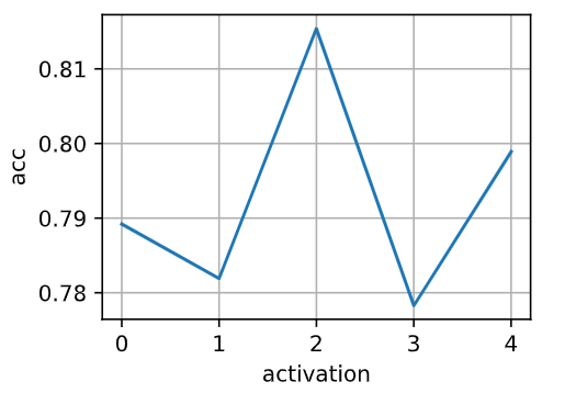
8. Try out different activation functions. Which one works best?

Tanh seems working best among these activation functions in this project.

class ActMLP(d2l.Classifier):
    def __init__(self, num_outputs, num_hiddens, lr, act=act):
        super().__init__()
        self.save_hyperparameters()
        self.net = nn.Sequential(nn.Flatten(), nn.LazyLinear(num_hiddens),
                                 nn.ReLU(), nn.LazyLinear(num_outputs))
        
def stat_act(act, data):
    model = ActMLP(num_outputs=10, num_hiddens=256, lr=0.1, act=act)
    trainer = d2l.Trainer(max_epochs=10, plot_flag=False)
    trainer.fit(model, data)
    y_hat = model(data.val.data.type(torch.float32))
    return model.accuracy(y_hat,data.val.targets).item()

acts = [nn.ReLU(),nn.Sigmoid(), nn.Tanh(),nn.LeakyReLU(negative_slope=0.01),nn.PReLU(num_parameters=1)]
accs = []
for act in tqdm(acts):
    accs.append(stat_act(act, data))

100%|██████████| 5/5 [12:36<00:00, 151.23s/it]

d2l.plot(range(len(acts)),accs[-len(lrs):],'activation','acc')

9. Is there a difference between weight initializations of the network? Does it matter?

Yes, there is a significant difference between weight initializations in a neural network, and it does matter. Weight initialization plays a crucial role in the convergence speed and stability of training, as well as the overall performance of a neural network.

Different weight initializations can lead to different learning dynamics during training, affect the optimization process, and impact the network’s ability to generalize to new data. Here are a few key points to consider:

1. Vanishing and Exploding Gradients:
   Poor weight initialization can lead to vanishing or exploding gradients, where the gradients become very small or very large as they are backpropagated through the network during training. This can slow down or hinder the convergence of the optimization process.

2. Convergence Speed:
   Proper weight initialization can help the network converge to a solution faster. Well-initialized networks tend to start with a better “starting point” in the optimization landscape, allowing the network to find a good solution more quickly.

3. Stability and Regularization:
   Certain weight initializations can act as implicit forms of regularization. For example, using a proper initialization can help prevent the network from immediately fitting noise in the training data.

4. Activation Functions:
   Different activation functions may require different weight initialization methods to ensure their effective usage. For example, the choice of initialization for a ReLU-based network might differ from that of a network using sigmoid activations.

5. Network Capacity and Depth:
   The choice of weight initialization may vary with the complexity of the network architecture. Deep networks might require more careful initialization due to the vanishing/exploding gradient problem.

6. Transfer Learning:
   Pre-trained models often come with their own weight initializations. Using these pre-trained weights can help in transfer learning tasks, as the network starts with features that are already useful for a related task.

Common weight initialization methods include Xavier/Glorot initialization, He initialization, uniform initialization, and normal initialization. The specific choice of initialization method depends on the network architecture, the activation functions used, and the problem domain.

In summary, weight initialization is not a trivial step in neural network training. Careful consideration and experimentation with different initialization methods can greatly impact the model’s convergence, training stability, and final performance.

import torch.nn.init as init


def init_xavier(module):
    if isinstance(module, nn.LazyLinear):
        init.xavier_uniform(module.weight)
        if module.bias is not None:
            init.constant_(module.bias, 0)
            
def init_uniform(module):
    if isinstance(module, nn.LazyLinear):
        init.uniform_(module.weight)
        if module.bias is not None:
            init.constant_(module.bias, 0)
            
def init_normal(module):
    if isinstance(module, nn.LazyLinear):
        init.normal_(module.weight)
        if module.bias is not None:
            init.constant_(module.bias, 0)
            
        
def stat_init(init_f, data):
    model = MLP(num_outputs=10, num_hiddens=256, lr=0.1)
    model.apply(init_f)
    trainer = d2l.Trainer(max_epochs=10, plot_flag=True)
    trainer.fit(model, data)
    y_hat = model(data.val.data.type(torch.float32))
    return model.accuracy(y_hat,data.val.targets).item()

inits = [init_xavier,init_uniform,init_normal]
accs = []
for i in tqdm(inits):
    accs.append(stat_init(i, data))
d2l.plot(list(range(len(inits))),accs[-len(inits):],'initializations','acc')

Reference

1. https://d2l.ai/chapter_multilayer-perceptrons/mlp-implementation.html