github:
https://github.com/pandalabme/d2l/tree/main/exercises

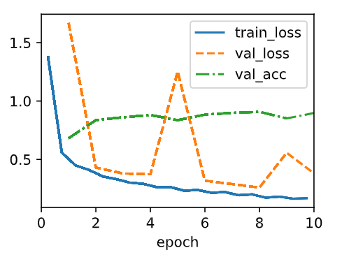
1. Increase the number of stages to four. Can you design a deeper RegNetX that performs better?

import torch
import torch.nn as nn
from torch.nn import functional as F
import sys
sys.path.append('/home/jovyan/work/d2l_solutions/notebooks/exercises/d2l_utils/')
import d2l
from torchsummary import summary

class AnyNet(d2l.Classifier):
    def stem(self, num_channels):
        return nn.Sequential(
            nn.LazyConv2d(num_channels, kernel_size=3, stride=2, padding=1),
            nn.LazyBatchNorm2d(), nn.ReLU())
    def stage(self, depth, num_channels, groups, bot_mul):
        blk = []
        for i in range(depth):
            if i == 0:
                blk.append(d2l.ResNeXtBlock(num_channels, groups, bot_mul,
                    use_1x1conv=True, strides=2))
            else:
                blk.append(d2l.ResNeXtBlock(num_channels, groups, bot_mul))
        return nn.Sequential(*blk)
    
    def __init__(self, arch, stem_channels, lr=0.1, num_classes=10):
        super(AnyNet, self).__init__()
        self.save_hyperparameters()
        self.net = nn.Sequential(self.stem(stem_channels))
        for i, s in enumerate(arch):
            self.net.add_module(f'stage{i+1}', self.stage(*s))
        self.net.add_module('head', nn.Sequential(
            nn.AdaptiveAvgPool2d((1, 1)), nn.Flatten(),
            nn.LazyLinear(num_classes)))
        self.net.apply(d2l.init_cnn)
        
class RegNetX32(AnyNet):
    def __init__(self, lr=0.1, num_classes=10):
        stem_channels, groups, bot_mul = 32, 16, 1
        depths, channels = (4, 6, 8, 16), (32, 80, 128, 256)
        super().__init__(
            # ((depths[0], channels[0], groups, bot_mul),
            #  (depths[1], channels[1], groups, bot_mul)),
            [(depths[i], channels[i], groups, bot_mul) for i in range(len(depths))],
            stem_channels, lr, num_classes)

model = RegNetX32(lr=0.05)
# summary(model,(1,224,224))
trainer = d2l.Trainer(max_epochs=10, num_gpus=1)
data = d2l.FashionMNIST(batch_size=128, resize=(224, 224))
trainer.fit(model, data)

2. De-ResNeXt-ify RegNets by replacing the ResNeXt block with the ResNet block. How does your new model perform?

class DeAnyNet(d2l.Classifier):
    def stem(self, num_channels):
        return nn.Sequential(
            nn.LazyConv2d(num_channels, kernel_size=3, stride=2, padding=1),
            nn.LazyBatchNorm2d(), nn.ReLU())
    def stage(self, depth, num_channels):
        blk = []
        for i in range(depth):
            if i == 0:
                blk.append(d2l.Residual(num_channels, use_1x1conv=True, strides=2))
            else:
                blk.append(d2l.Residual(num_channels))
        return nn.Sequential(*blk)
    
    def __init__(self, arch, stem_channels, lr=0.1, num_classes=10):
        super().__init__()
        self.save_hyperparameters()
        self.net = nn.Sequential(self.stem(stem_channels))
        for i, s in enumerate(arch):
            self.net.add_module(f'stage{i+1}', self.stage(*s))
        self.net.add_module('head', nn.Sequential(
            nn.AdaptiveAvgPool2d((1, 1)), nn.Flatten(),
            nn.LazyLinear(num_classes)))
        self.net.apply(d2l.init_cnn)
        
class DeResNeXt(DeAnyNet):
    def __init__(self, lr=0.1, num_classes=10):
        stem_channels, groups, bot_mul = 32, 16, 1
        depths, channels = (5, 6), (32, 80)
        super().__init__(
            ((depths[0], channels[0]),
             (depths[1], channels[1])),
            stem_channels, lr, num_classes)

model = DeResNeXt(lr=0.05)
trainer = d2l.Trainer(max_epochs=10, num_gpus=1)
trainer.fit(model, data)

3. Implement multiple instances of a “VioNet” family by violating the design principles of RegNetX. How do they perform? Which of (d_i,c_i,g_i,b_i) is the most important factor?

class VioNet(AnyNet):
    def __init__(self, lr=0.1, num_classes=10, depths=(4, 6), channels=(32, 80),
                 stem_channels=32, groups=(16, 16), bot_mul=(1, 1)):
        super().__init__(
            [(depths[i], channels[i], groups[i], bot_mul[i]) for i in range(len(depths))],
            stem_channels, lr, num_classes)

VioNet_d = VioNet(depths=(6, 4))
trainer = d2l.Trainer(max_epochs=10, num_gpus=1)
trainer.fit(VioNet_d, data)

VioNet_c = VioNet(channels=(80, 32))
trainer = d2l.Trainer(max_epochs=10, num_gpus=1)
trainer.fit(VioNet_c, data)

VioNet_g = VioNet(groups=(16, 32))
trainer = d2l.Trainer(max_epochs=10, num_gpus=1)
trainer.fit(VioNet_g, data)

VioNet_b = VioNet(bot_mul=(1, 2))
trainer = d2l.Trainer(max_epochs=10, num_gpus=1)
trainer.fit(VioNet_b, data)

4. Your goal is to design the “perfect” MLP. Can you use the design principles introduced above to find good architectures? Is it possible to extrapolate from small to large networks?

Designing the “perfect” Multilayer Perceptron (MLP) involves careful consideration of architectural choices to achieve high performance on a specific task. The paper “On Network Design Spaces for Visual Recognition” discusses several design principles that can be applied to create effective neural network architectures for visual recognition. Here’s how you can use these design principles to design an effective MLP:

1. Depth and Width:

   • Depth: Experiment with different numbers of layers (depth) in your MLP. Start with a moderate depth and gradually increase it while monitoring performance. Deep networks can capture complex features but may require techniques like skip connections (ResNets) to mitigate vanishing gradients.
   • Width: Vary the number of neurons (width) in each layer. Wider layers can capture more complex patterns, but they may also increase the risk of overfitting. You can use techniques like dropout or batch normalization to regularize the network.

2. Skip Connections:

   • Consider adding skip connections between layers, similar to Residual Networks (ResNets). These connections can help alleviate vanishing gradient problems and enable the training of very deep networks.

3. Kernel Sizes:

   • Experiment with different kernel sizes for convolutional layers or different numbers of neurons in fully connected layers. Smaller kernels can capture fine details, while larger kernels can capture broader patterns.

4. Pooling Strategies:

   • Use different pooling strategies like max-pooling or average pooling to downsample feature maps. The choice of pooling can affect the invariance and spatial resolution of the learned features.

5. Normalization:

   • Incorporate batch normalization layers to stabilize training and improve convergence. Batch normalization can also act as a regularizer.

6. Activation Functions:

   • Experiment with different activation functions like ReLU, Leaky ReLU, or variants like Swish. The choice of activation function can affect the network’s capacity to model complex data distributions.

7. Dropout:

   • Apply dropout with varying dropout rates to prevent overfitting. You can selectively apply dropout to certain layers or neurons based on their importance.

8. Initialization:

   • Use appropriate weight initialization techniques such as Xavier/Glorot initialization or He initialization. Proper initialization can expedite training and improve convergence.

9. Normalization Layers:

   • Experiment with layer normalization or group normalization in addition to batch normalization to see if they offer advantages in your specific task.

10. Optimizers and Learning Rates:

    • Choose appropriate optimizers (e.g., Adam, SGD) and learning rate schedules. Learning rate schedules like learning rate annealing or cyclic learning rates can help in training.

11. Regularization Techniques:

    • Consider L1 and L2 regularization to control the complexity of the model and prevent overfitting. You can also explore more advanced regularization techniques like dropout, weight decay, or early stopping.

12. Task-Specific Architectures:

    • Tailor your MLP architecture to the specific task. For example, use a final softmax layer for classification tasks or a linear layer for regression tasks.

13. Ensemble Learning:

    • Experiment with ensemble methods to combine multiple MLPs for improved performance and robustness.

14. Hyperparameter Search:

    • Perform systematic hyperparameter tuning using techniques like grid search or random search to find the best combination of hyperparameters.

15. Transfer Learning:

    • Consider using transfer learning by initializing your MLP with pretrained weights from a model trained on a related task. Fine-tuning the network on your specific task can significantly boost performance.

16. Data Augmentation:

    • Apply data augmentation techniques to increase the effective size of your training dataset and improve the model’s generalization.

17. Regularly Evaluate Performance:

    • Continuously monitor and evaluate the model’s performance on a validation dataset. Adjust architectural choices based on performance feedback.

Remember that designing the “perfect” MLP involves an iterative process of experimentation, evaluation, and refinement. The choice of architecture and design principles should align with the specific requirements and constraints of your task and dataset.

Reference

1. https://d2l.ai/chapter_convolutional-modern/cnn-design.html