github:
https://github.com/pandalabme/d2l/tree/main/exercises

1. Should we remove the bias parameter from the fully connected layer or the convolutional layer before the batch normalization? Why?

Batch normalization is a technique that helps stabilize and accelerate the training of deep neural networks. It normalizes the activations within a layer by subtracting the mean and dividing by the standard deviation of the mini-batch. The normalized activations are then scaled and shifted using learnable parameters: the scale (gamma) and shift (beta) parameters.

When using batch normalization, it’s generally recommended to remove the bias parameter from the fully connected (linear) layer before applying batch normalization. This recommendation comes from the idea that the normalization process already includes shifting the activations with the beta parameter of batch normalization. Adding an additional bias term can introduce redundancy and might negatively impact the learning process.

For convolutional layers, the use of bias parameters is less clear-cut. Whether to use bias parameters before batch normalization in convolutional layers depends on your specific use case and the design choices you are making.

Here’s a general guideline for both cases:

1. Fully Connected (Linear) Layer:

   • Remove Bias: It’s recommended to remove the bias parameter from the fully connected layer before applying batch normalization. This helps avoid the potential redundancy between the bias and beta parameters of batch normalization.

2. Convolutional Layer:

   • With Bias: Some architectures and setups use bias parameters in convolutional layers before batch normalization. The bias parameter can still provide flexibility in modeling, especially in the early stages of the network.
   • Without Bias: If you decide to remove the bias parameter from convolutional layers before batch normalization, you’re essentially letting batch normalization handle both the shifting and scaling of the activations.

Remember that the effectiveness of these choices can also depend on the specific architecture, dataset, and optimization process you’re using. It’s often a good idea to experiment with different configurations to find the best setup for your particular use case.

In summary, for fully connected layers, it’s generally recommended to remove the bias parameter before applying batch normalization. For convolutional layers, you have some flexibility and can choose to include or exclude bias parameters based on your design choices and performance considerations.

2. Compare the learning rates for LeNet with and without batch normalization.

import sys
import torch.nn as nn
import torch
import warnings
sys.path.append('/home/jovyan/work/d2l_solutions/notebooks/exercises/d2l_utils/')
import d2l
from torchsummary import summary
warnings.filterwarnings("ignore")

class LeNet(d2l.Classifier):  #@save
    """The LeNet-5 model."""
    def __init__(self, lr=0.1, num_classes=10):
        super().__init__()
        self.save_hyperparameters()
        self.net = nn.Sequential(
            nn.LazyConv2d(6, kernel_size=5, padding=2), nn.Sigmoid(),
            nn.AvgPool2d(kernel_size=2, stride=2),
            nn.LazyConv2d(16, kernel_size=5), nn.Sigmoid(),
            nn.AvgPool2d(kernel_size=2, stride=2),
            nn.Flatten(),
            nn.LazyLinear(120), nn.Sigmoid(),
            nn.LazyLinear(84), nn.Sigmoid(),
            nn.LazyLinear(num_classes))
        
class BNLeNet(d2l.Classifier):
    def __init__(self, lr=0.1, num_classes=10):
        super().__init__()
        self.save_hyperparameters()
        self.net = nn.Sequential(
            nn.LazyConv2d(6, kernel_size=5), nn.LazyBatchNorm2d(),
            nn.Sigmoid(), nn.AvgPool2d(kernel_size=2, stride=2),
            nn.LazyConv2d(16, kernel_size=5), nn.LazyBatchNorm2d(),
            nn.Sigmoid(), nn.AvgPool2d(kernel_size=2, stride=2),
            nn.Flatten(), nn.LazyLinear(120), nn.LazyBatchNorm1d(),
            nn.Sigmoid(), nn.LazyLinear(84), nn.LazyBatchNorm1d(),
            nn.Sigmoid(), nn.LazyLinear(num_classes))
        
def stat_model_acc(model, data, plot_flag):
    model.apply_init([next(iter(data.get_dataloader(True)))[0]], d2l.init_cnn)
    trainer = d2l.Trainer(max_epochs=10, num_gpus=1,plot_flag=plot_flag)
    trainer.fit(model, data)
    X,y = next(iter(data.get_dataloader(False)))
    X = X.to('cuda')
    y = y.to('cuda')
    y_hat = model(X) 
    return model.accuracy(y_hat,y).item()

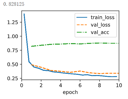
2.1 Plot the increase in validation accuracy.

data = d2l.FashionMNIST(batch_size=128)
lr_list = [0.001,0.01,0.03,0.1,0.3]
le_accs= []
ble_accs = []
for lr in lr_list[:1]:
    le = LeNet(lr=lr)
    ble = BNLeNet(lr=lr)
    le_acc.append(stat_model_acc(le, data, False))
    ble_acc.append(stat_model_acc(ble, data, False))

2.2 How large can you make the learning rate before the optimization fails in both cases?

3. Do we need batch normalization in every layer? Experiment with it.

Whether to apply batch normalization in every layer of a neural network is not a strict rule but a design choice that depends on the specific problem, architecture, and training dynamics. The decision can impact the model’s convergence, performance, and training stability. Here are some considerations to help you decide:

Advantages of Batch Normalization in Every Layer:

1. Stabilized Training: Applying batch normalization in every layer helps stabilize training by normalizing activations and reducing internal covariate shifts, which can lead to faster convergence and more stable gradient propagation.

2. Regularization: Batch normalization has an inherent regularization effect, which can help prevent overfitting. Applying it in every layer might provide consistent regularization throughout the network.

3. Deeper Architectures: For very deep networks, applying batch normalization in every layer can help mitigate gradient vanishing/exploding problems, enabling the training of even deeper models.

4. Less Sensitive to Initialization: Batch normalization can reduce the sensitivity to weight initialization, allowing you to use larger learning rates and more aggressive optimization techniques.

Considerations Against Batch Normalization in Every Layer:

1. Reduced Model Capacity: Batch normalization can suppress the network’s capacity to fit the training data. Applying it too frequently might lead to underfitting, especially in smaller models.

2. Slower Training: Adding batch normalization to every layer increases computational overhead, which might slow down training, especially on hardware with limited resources.

3. Loss of Expressiveness: Excessive normalization can remove useful information from activations, potentially limiting the model’s expressiveness. It can also hinder the model’s ability to memorize certain patterns, which could be desirable in some scenarios.

4. Unstable for Very Small Batches: Batch normalization relies on batch statistics, which can be unstable for very small batches. In such cases, using batch normalization in every layer might lead to poor performance.

Guidelines and Best Practices:

1. Experiment: It’s recommended to experiment with different configurations, including applying batch normalization selectively or in every layer. Test the impact on validation performance, convergence speed, and generalization.

2. Network Depth: Deeper networks tend to benefit more from batch normalization in every layer due to the vanishing gradient problem. For shallower networks, you might achieve good results with selective application.

3. Use Validation: Monitor validation performance during training to detect potential overfitting caused by excessive batch normalization.

4. Small Datasets: For small datasets, you might need to be more cautious with normalization. Experiment with validation performance to find the right balance.

5. Different Architectures: Different architectures might respond differently to batch normalization. What works for one architecture might not work optimally for another.

In conclusion, while applying batch normalization in every layer can have benefits, it’s important to consider the trade-offs and experiment with different configurations. The choice depends on your specific use case, the architecture of your model, the dataset, and computational constraints.

4. Implement a “lite” version of batch normalization that only removes the mean, or alternatively one that only removes the variance. How does it behave?

def lite_batch_norm(X, gamma, beta, moving_mean, moving_var, eps, momentum, mean_flag):
    # Use is_grad_enabled to determine whether we are in training mode
    if not torch.is_grad_enabled():
        # In prediction mode, use mean and variance obtained by moving average
        if mean_flag:
            X_hat = X - moving_mean
        else:
            X_hat = X / torch.sqrt(moving_var + eps)
    else:
        assert len(X.shape) in (2, 4)
        if len(X.shape) == 2:
            # When using a fully connected layer, calculate the mean and
            # variance on the feature dimension
            mean = X.mean(dim=0)
            var = ((X - mean) ** 2).mean(dim=0)
        else:
            # When using a two-dimensional convolutional layer, calculate the
            # mean and variance on the channel dimension (axis=1). Here we
            # need to maintain the shape of X, so that the broadcasting
            # operation can be carried out later
            mean = X.mean(dim=(0, 2, 3), keepdim=True)
            var = ((X - mean) ** 2).mean(dim=(0, 2, 3), keepdim=True)
        # In training mode, the current mean and variance are used
        if mean_flag:
            X_hat = X - mean
        else:
            X_hat = X / torch.sqrt(moving_var + eps)
        # Update the mean and variance using moving average
        moving_mean = (1.0 - momentum) * moving_mean + momentum * mean
        moving_var = (1.0 - momentum) * moving_var + momentum * var
    Y = gamma * X_hat + beta  # Scale and shift
    return Y, moving_mean.data, moving_var.data

class LiteBatchNorm(nn.Module):
    # num_features: the number of outputs for a fully connected layer or the
    # number of output channels for a convolutional layer. num_dims: 2 for a
    # fully connected layer and 4 for a convolutional layer
    def __init__(self, num_features, num_dims, mean_flag=True):
        super().__init__()
        if num_dims == 2:
            shape = (1, num_features)
        else:
            shape = (1, num_features, 1, 1)
        # The scale parameter and the shift parameter (model parameters) are
        # initialized to 1 and 0, respectively
        self.gamma = nn.Parameter(torch.ones(shape))
        self.beta = nn.Parameter(torch.zeros(shape))
        # The variables that are not model parameters are initialized to 0 and
        # 1
        self.moving_mean = torch.zeros(shape)
        self.moving_var = torch.ones(shape)
        self.mean_flag = mean_flag

    def forward(self, X):
        # If X is not on the main memory, copy moving_mean and moving_var to
        # the device where X is located
        if self.moving_mean.device != X.device:
            self.moving_mean = self.moving_mean.to(X.device)
            self.moving_var = self.moving_var.to(X.device)
        # Save the updated moving_mean and moving_var
        Y, self.moving_mean, self.moving_var = batch_norm(
            X, self.gamma, self.beta, self.moving_mean,
            self.moving_var, eps=1e-5, momentum=0.1, mean_flag=self.mean_flag)
        return Y

    
class LiteBNLeNetScratch(d2l.Classifier):
    def __init__(self, lr=0.1, num_classes=10, mean_flag=True):
        super().__init__()
        self.save_hyperparameters()
        self.net = nn.Sequential(
            nn.LazyConv2d(6, kernel_size=5), LiteBatchNorm(6, num_dims=4, mean_flag=mean_flag),
            nn.Sigmoid(), nn.AvgPool2d(kernel_size=2, stride=2),
            nn.LazyConv2d(16, kernel_size=5), LiteBatchNorm(16, num_dims=4, mean_flag=mean_flag),
            nn.Sigmoid(), nn.AvgPool2d(kernel_size=2, stride=2),
            nn.Flatten(), nn.LazyLinear(120),
            LiteBatchNorm(120, num_dims=2, mean_flag=mean_flag), nn.Sigmoid(), nn.LazyLinear(84),
            LiteBatchNorm(84, num_dims=2, mean_flag=mean_flag), nn.Sigmoid(),
            nn.LazyLinear(num_classes))

model = LiteBNLeNetScratch(lr=0.1)
model.apply_init([next(iter(data.get_dataloader(True)))[0]], d2l.init_cnn)
trainer = d2l.Trainer(max_epochs=10, num_gpus=1)
trainer.fit(model, data)
X,y = next(iter(data.get_dataloader(False)))
X = X.to('cuda')
y = y.to('cuda')
y_hat = model(X)
model.accuracy(y_hat,y).item()

model = LiteBNLeNetScratch(lr=0.1,mean_flag=False)
model.apply_init([next(iter(data.get_dataloader(True)))[0]], d2l.init_cnn)
trainer = d2l.Trainer(max_epochs=10, num_gpus=1)
trainer.fit(model, data)
X,y = next(iter(data.get_dataloader(False)))
X = X.to('cuda')
y = y.to('cuda')
y_hat = model(X)
model.accuracy(y_hat,y).item()

5. Fix the parameters beta and gamma. Observe and analyze the results.

class FixedBatchNorm(nn.Module):
    # num_features: the number of outputs for a fully connected layer or the
    # number of output channels for a convolutional layer. num_dims: 2 for a
    # fully connected layer and 4 for a convolutional layer
    def __init__(self, num_features, num_dims, beta=None, gamma=None):
        super().__init__()
        if num_dims == 2:
            shape = (1, num_features)
        else:
            shape = (1, num_features, 1, 1)
        # The scale parameter and the shift parameter (model parameters) are
        # initialized to 1 and 0, respectively
        self.gamma = torch.ones(shape) if gamma is None else gamma
        self.beta = torch.zeros(shape) if beta is None else beta
        # The variables that are not model parameters are initialized to 0 and
        # 1
        self.moving_mean = torch.zeros(shape)
        self.moving_var = torch.ones(shape)
        self.mean_flag = mean_flag

    def forward(self, X):
        # If X is not on the main memory, copy moving_mean and moving_var to
        # the device where X is located
        if self.moving_mean.device != X.device:
            self.moving_mean = self.moving_mean.to(X.device)
            self.moving_var = self.moving_var.to(X.device)
        # Save the updated moving_mean and moving_var
        Y, self.moving_mean, self.moving_var = batch_norm(
            X, self.gamma, self.beta, self.moving_mean,
            self.moving_var, eps=1e-5, momentum=0.1, mean_flag=self.mean_flag)
        return Y

    
class FixedBNLeNetScratch(d2l.Classifier):
    def __init__(self, lr=0.1, num_classes=10, beta=None, gamma=None):
        super().__init__()
        self.save_hyperparameters()
        self.net = nn.Sequential(
            nn.LazyConv2d(6, kernel_size=5), FixedBatchNorm(6, num_dims=4, beta=beta, gamma=gamma),
            nn.Sigmoid(), nn.AvgPool2d(kernel_size=2, stride=2),
            nn.LazyConv2d(16, kernel_size=5), FixedBatchNorm(16, num_dims=4, beta=beta, gamma=gamma),
            nn.Sigmoid(), nn.AvgPool2d(kernel_size=2, stride=2),
            nn.Flatten(), nn.LazyLinear(120),
            FixedBatchNorm(120, num_dims=2, beta=beta, gamma=gamma), nn.Sigmoid(), nn.LazyLinear(84),
            FixedBatchNorm(84, num_dims=2, beta=beta, gamma=gamma), nn.Sigmoid(),
            nn.LazyLinear(num_classes))

6. Can you replace dropout by batch normalization? How does the behavior change?

Dropout and batch normalization are two different techniques used for regularization in neural networks. While they both aim to prevent overfitting, they operate in distinct ways. Dropout involves randomly dropping out units (neurons) during training, while batch normalization normalizes activations in each layer. They serve different purposes, and replacing one with the other may not yield the same results.

7. Research ideas: think of other normalization transforms that you can apply:

7.1 Can you apply the probability integral transform?

def gen_sort_cdf(data):
    sorts = []
    cdfs = []
    for i in range(data.shape[1]):
        sort = np.sort(data[:, i])
        cdf = np.arange(1, len(sort) + 1) / len(sort)
        sorts.append(torch.tensor(sort).reshape(-1,1))
        cdfs.append(torch.tensor(cdf).reshape(-1,1))
    return torch.cat(sorts, dim=1), torch.cat(cdfs, dim=1)

def pit_col(sorted_data, cdf_values, data):
    # sorted_data = np.sort(org_data)
    # cdf_values = np.arange(1, len(sorted_data) + 1) / len(sorted_data)
    transformed_data = np.interp(data, sorted_data, cdf_values)
    return 

def pit(sorted_data, cdf_values, data):
    return torch.cat([pit_col(sorted_data[:,i], cdf_values[:,i], data[:, i]) for i in range(data.shape[1])], dim=1)

def batch_pit_norm(X, gamma, beta, moving_sorted, moving_cdf, momentum):
    # Use is_grad_enabled to determine whether we are in training mode
    assert len(X.shape) in (2, 4)
    shape  = X.shape
    if len(shape) == 4:
        X = torch.transpose(X,0,1).reshape(shape[1],-1)
    if not torch.is_grad_enabled():
        # In prediction mode, use mean and variance obtained by moving average
        X_hat = pit(moving_sorted, moving_cdf, cdfs, X)
    else:
        sorts, cdfs = gen_sort_cdf(data)
        X_hat = pit(sorts, cdfs, X)
        moving_sorted = (1.0 - momentum) * moving_sorted + momentum * sorts
        moving_cdf = (1.0 - momentum) * moving_cdf + momentum * cdfs
    X_hat = X.reshape(shape)
        # Update the mean and variance using moving average
    Y = gamma * X_hat + beta  # Scale and shift
    return Y, moving_sorted, moving_cdf

class PitBatchNorm(nn.Module):
    # num_features: the number of outputs for a fully connected layer or the
    # number of output channels for a convolutional layer. num_dims: 2 for a
    # fully connected layer and 4 for a convolutional layer
    def __init__(self, num_features, num_dims):
        super().__init__()
        if num_dims == 2:
            shape = (1, num_features)
        else:
            shape = (1, num_features, 1, 1)
        # The scale parameter and the shift parameter (model parameters) are
        # initialized to 1 and 0, respectively
        self.gamma = nn.Parameter(torch.ones(shape))
        self.beta = nn.Parameter(torch.zeros(shape))
        # The variables that are not model parameters are initialized to 0 
        self.moving_sorted = torch.zeros(shape)
        self.moving_cdf = torch.zeros(shape)
       
    def forward(self, X):
        # If X is not on the main memory, copy moving_mean and moving_var to
        # the device where X is located
        if self.moving_sorted.device != X.device:
            self.moving_sorted = self.moving_sorted.to(X.device)
            self.moving_cdf = self.moving_cdf.to(X.device)
        # Save the updated moving_mean and moving_var
        Y, self.moving_sorted, self.moving_cdf = batch_pit_norm(
            X, self.gamma, self.beta, self.moving_sorted,
            self.moving_cdf, momentum=0.1)
        return Y

    
class PitBNLeNetScratch(d2l.Classifier):
    def __init__(self, lr=0.1, num_classes=10, mean_flag=True):
        super().__init__()
        self.save_hyperparameters()
        self.net = nn.Sequential(
            nn.LazyConv2d(6, kernel_size=5), PitBatchNorm(6, num_dims=4),
            nn.Sigmoid(), nn.AvgPool2d(kernel_size=2, stride=2),
            nn.LazyConv2d(16, kernel_size=5), PitBatchNorm(6, num_dims=4),
            nn.Sigmoid(), nn.AvgPool2d(kernel_size=2, stride=2),
            nn.Flatten(), nn.LazyLinear(120),
            PitBatchNorm(6, num_dims=4), nn.Sigmoid(), nn.LazyLinear(84),
            PitBatchNorm(6, num_dims=4), nn.Sigmoid(),
            nn.LazyLinear(num_classes))

# model = PitBNLeNetScratch(lr=0.1)

7.2 Can you use a full-rank covariance estimate? Why should you probably not do that?

Using a full-rank covariance estimate instead of the standard normalization transform (mean and variance) in batch normalization is an interesting idea, but it’s not typically recommended for several reasons:

1. Computational Complexity: Computing the full-rank covariance matrix is more computationally expensive compared to calculating the mean and variance. The covariance matrix has quadratic complexity with respect to the input dimensions, while mean and variance calculations are linear. This added complexity can slow down training significantly.

2. Dimension Mismatch: Batch normalization is applied independently to each channel (feature) in the input. When computing the covariance matrix, you would typically need to consider interactions between different channels, which could lead to a higher-dimensional covariance matrix. This might not work well for the normalization purposes of batch normalization.

3. Instability: Computing the full-rank covariance matrix on small batch sizes or when the data has high dimensionality can lead to numerical instability and ill-conditioned covariance matrices. Regularization or other techniques might be needed to ensure numerical stability.

4. Overfitting: Using a full-rank covariance matrix could introduce additional learnable parameters. This might lead to overfitting, especially if the network is not large enough or the dataset is not sufficiently diverse.

5. Loss of Orthogonality: One of the benefits of batch normalization is that it maintains the orthogonality between the weight updates and the gradient updates during backpropagation. Introducing a full-rank covariance matrix might break this orthogonality, leading to slower convergence or training instability.

6. Normalization Properties: Batch normalization is designed to normalize each channel’s activations independently. A full-rank covariance estimate might introduce interdependencies between channels, which could disrupt the normalization properties.

7. Lack of Empirical Support: The standard batch normalization approach using mean and variance has been empirically proven to work well across a wide range of network architectures and tasks. There’s less evidence supporting the effectiveness of using a full-rank covariance estimate.

In summary, while the idea of using a full-rank covariance matrix in batch normalization is intriguing, it’s not commonly used due to the potential drawbacks in terms of computational complexity, instability, and the mismatch between batch normalization’s design principles and the properties of a full-rank covariance matrix. The standard normalization transforms (mean and variance) have been well-tested and proven to be effective in stabilizing and accelerating the training of neural networks.

def batch_frcov_norm(X, gamma, beta, moving_cov_matrix, momentum):
    # Use is_grad_enabled to determine whether we are in training mode
    assert len(X.shape) in (2, 4)
    shape  = X.shape
    if len(shape) == 4:
        X = torch.transpose(X,0,1).reshape(shape[1],-1)
    if not torch.is_grad_enabled():
        # In prediction mode, use mean and variance obtained by moving average
        eigenvalues, eigenvectors = torch.linalg.eig(moving_cov_matrix)
        X_hat = X @ eigenvectors.type(torch.float32)
    else:
        centered_data = X - X.mean(dim=0)
        cov_matrix = (centered_data.conj().T @ centered_data) / (X.shape[0] - 1)
        eigenvalues, eigenvectors = torch.linalg.eig(cov_matrix)
        X_hat = X @ eigenvectors.type(torch.float32)
        moving_cov_matrix = (1.0 - momentum) * moving_cov_matrix + momentum * cov_matrix
    X_hat = X.reshape(shape)
        # Update the mean and variance using moving average
    Y = gamma * X_hat + beta  # Scale and shift
    return Y, moving_cov_matrix

class FrcovBatchNorm(nn.Module):
    # num_features: the number of outputs for a fully connected layer or the
    # number of output channels for a convolutional layer. num_dims: 2 for a
    # fully connected layer and 4 for a convolutional layer
    def __init__(self, num_features, num_dims):
        super().__init__()
        if num_dims == 2:
            shape = (1, num_features)
        else:
            shape = (1, num_features, 1, 1)
        # The scale parameter and the shift parameter (model parameters) are
        # initialized to 1 and 0, respectively
        self.gamma = nn.Parameter(torch.ones(shape))
        self.beta = nn.Parameter(torch.zeros(shape))
        # The variables that are not model parameters are initialized to 0 
        self.moving_cov_matrix = torch.zeros(shape)
       
    def forward(self, X):
        # If X is not on the main memory, copy moving_mean and moving_var to
        # the device where X is located
        if self.moving_cov_matrix.device != X.device:
            self.moving_cov_matrix = self.moving_cov_matrix.to(X.device)
        # Save the updated moving_mean and moving_var
        Y, self.moving_cov_matrix = batch_frcov_norm(
            X, self.gamma, self.beta, self.moving_cov_matrix,
            momentum=0.1)
        return Y

    
class FrcovBNLeNetScratch(d2l.Classifier):
    def __init__(self, lr=0.1, num_classes=10, mean_flag=True):
        super().__init__()
        self.save_hyperparameters()
        self.net = nn.Sequential(
            nn.LazyConv2d(6, kernel_size=5), FrcovBatchNorm(6, num_dims=4),
            nn.Sigmoid(), nn.AvgPool2d(kernel_size=2, stride=2),
            nn.LazyConv2d(16, kernel_size=5), FrcovBatchNorm(6, num_dims=4),
            nn.Sigmoid(), nn.AvgPool2d(kernel_size=2, stride=2),
            nn.Flatten(), nn.LazyLinear(120),
            FrcovBatchNorm(6, num_dims=4), nn.Sigmoid(), nn.LazyLinear(84),
            FrcovBatchNorm(6, num_dims=4), nn.Sigmoid(),
            nn.LazyLinear(num_classes))

# model = FrcovBNLeNetScratch(lr=0.1)

7.3 Can you use other compact matrix variants (block-diagonal, low-displacement rank, Monarch, etc.)?

def batch_bdcov_norm(X, gamma, beta, moving_cov_matrix, momentum):
    # Use is_grad_enabled to determine whether we are in training mode
    assert len(X.shape) in (2, 4)
    shape  = X.shape
    if len(shape) == 4:
        X = torch.transpose(X,0,1).reshape(shape[1],-1)
    if not torch.is_grad_enabled():
        # In prediction mode, use mean and variance obtained by moving average
        diagonal_matrix = torch.diag_embed(moving_cov_matrix)
        block_diagonal_matrix = torch.sum(diagonal_matrix, dim=0)
        X_hat = X @ block_diagonal_matrix
    else:
        centered_data = X - X.mean(dim=0)
        cov_matrix = (centered_data.conj().T @ centered_data) / (X.shape[0] - 1)
        diagonal_matrix = torch.diag_embed(moving_cov_matrix)
        block_diagonal_matrix = torch.sum(diagonal_matrix, dim=0)
        X_hat = X @ block_diagonal_matrix
        moving_cov_matrix = (1.0 - momentum) * moving_cov_matrix + momentum * cov_matrix
    X_hat = X.reshape(shape)
        # Update the mean and variance using moving average
    Y = gamma * X_hat + beta  # Scale and shift
    return Y, moving_cov_matrix

class BdcovBatchNorm(nn.Module):
    # num_features: the number of outputs for a fully connected layer or the
    # number of output channels for a convolutional layer. num_dims: 2 for a
    # fully connected layer and 4 for a convolutional layer
    def __init__(self, num_features, num_dims):
        super().__init__()
        if num_dims == 2:
            shape = (1, num_features)
        else:
            shape = (1, num_features, 1, 1)
        # The scale parameter and the shift parameter (model parameters) are
        # initialized to 1 and 0, respectively
        self.gamma = nn.Parameter(torch.ones(shape))
        self.beta = nn.Parameter(torch.zeros(shape))
        # The variables that are not model parameters are initialized to 0 
        self.moving_cov_matrix = torch.zeros(shape)
       
    def forward(self, X):
        # If X is not on the main memory, copy moving_mean and moving_var to
        # the device where X is located
        if self.moving_cov_matrix.device != X.device:
            self.moving_cov_matrix = self.moving_cov_matrix.to(X.device)
        # Save the updated moving_mean and moving_var
        Y, self.moving_cov_matrix = batch_bdcov_norm(
            X, self.gamma, self.beta, self.moving_cov_matrix,
            momentum=0.1)
        return Y

    
class BdcovBNLeNetScratch(d2l.Classifier):
    def __init__(self, lr=0.1, num_classes=10, mean_flag=True):
        super().__init__()
        self.save_hyperparameters()
        self.net = nn.Sequential(
            nn.LazyConv2d(6, kernel_size=5), BdcovBatchNorm(6, num_dims=4),
            nn.Sigmoid(), nn.AvgPool2d(kernel_size=2, stride=2),
            nn.LazyConv2d(16, kernel_size=5), BdcovBatchNorm(6, num_dims=4),
            nn.Sigmoid(), nn.AvgPool2d(kernel_size=2, stride=2),
            nn.Flatten(), nn.LazyLinear(120),
            BdcovBatchNorm(6, num_dims=4), nn.Sigmoid(), nn.LazyLinear(84),
            BdcovBatchNorm(6, num_dims=4), nn.Sigmoid(),
            nn.LazyLinear(num_classes))

7.4 Does a sparsification compression act as a regularizer?

Yes, sparsification compression can act as a form of regularization in machine learning models. Sparsification refers to the process of converting certain weights or parameters in a model to zero, effectively creating a sparse representation. This process can have a regularizing effect on the model’s learning process and can help prevent overfitting.

Here’s how sparsification compression can act as a regularizer:

1. Reduced Model Complexity: Sparsification reduces the number of active parameters in the model, leading to a simpler model representation. This can help prevent the model from capturing noise in the training data and focusing on the most relevant features.

2. Prevention of Overfitting: A sparse model is less likely to overfit the training data because it has fewer degrees of freedom. Overfitting occurs when a model becomes too complex and fits noise in the training data, leading to poor generalization to unseen data. Sparsification helps mitigate this by limiting the model’s capacity to overfit.

3. Improved Generalization: Regularization techniques like sparsification often lead to improved generalization performance. By encouraging the model to focus on the most informative features, the model becomes more robust and performs better on new, unseen data.

4. Interpretability: Sparse models are often more interpretable because they highlight the most influential features. This can provide insights into which features are driving the model’s decisions, making it easier to understand and debug.

5. Efficiency: Sparse models are computationally more efficient, as they involve fewer computations during inference. This efficiency can be beneficial for deploying models to resource-constrained environments.

It’s important to note that while sparsification compression can provide regularization benefits, the degree of regularization depends on the extent of sparsity and the sparsification method used. Various techniques, such as L1 regularization (lasso), dropout, or techniques specific to neural network pruning, can be used to induce sparsity and act as regularization in different contexts. However, the exact regularization effect might vary based on the specific problem, dataset, and architecture.

7.5 Are there other projections (e.g., convex cone, symmetry group-specific transforms) that you can use?

Yes, there are several other types of projections and transforms that can be used in various mathematical and computational contexts. These projections are often used to achieve specific properties, structures, or constraints on data or mathematical objects. Here are a few examples:

1. Convex Cone Projection: Convex cones are sets of vectors that are closed under linear combinations with non-negative coefficients. Projecting onto a convex cone involves finding the point in the cone that is closest to a given vector. This kind of projection is often used in optimization problems where the solution must satisfy certain constraints.

2. Symmetry Group-Specific Transforms: In some applications, you might want to transform data or objects to respect specific symmetries. For example, in crystallography, Fourier transforms are used to reveal the symmetry of a crystal lattice. In image processing, you might use transforms that respect rotational or translational symmetries.

3. Orthogonal Projection: Orthogonal projection involves finding the closest point in a subspace to a given vector. This type of projection is commonly used in linear algebra and optimization, where you might want to find the best approximation of a vector within a subspace.

4. Quantization: Quantization is a projection-like operation used to map continuous values to a discrete set of values. It’s often used in signal processing and data compression to reduce the number of possible values while minimizing information loss.

5. Manifold Embedding: Manifold learning techniques aim to embed high-dimensional data into lower-dimensional spaces while preserving certain properties or structures. Techniques like Isomap, Locally Linear Embedding (LLE), and t-Distributed Stochastic Neighbor Embedding (t-SNE) are examples of such manifold embedding methods.

6. Orthogonal Procrustes Problem: In linear algebra, the Orthogonal Procrustes Problem involves finding an orthogonal transformation (rotation and reflection) that best aligns two sets of points. It’s often used in computer graphics, shape analysis, and alignment tasks.

These are just a few examples of the many types of projections and transforms used in various fields. The choice of projection or transform depends on the problem at hand and the specific properties or constraints you want to achieve.

Reference

1. https://d2l.ai/chapter_convolutional-modern/batch-norm.html