Introduction

Business Context

The ability to price an insurance quote properly has a significant impact on insurers' management decisions and financial statements. You are the chief data scientist at a new startup insurance company focusing on providing affordable insurance to millennials. You are tasked to assess the current state of insurance companies to see what factors large insurance providers charge premiums for. Fortunately for you, your company has compiled a dataset by surveying what people currently pay for insurance from large companies. Your findings will be used as the basis of developing your company's millenial car insurance offering.

Business Problem

Your task is to build a minimal model to predict the cost of insurance from the data set using various characteristics of a policyholder.

Analytical Context

The data resides in a CSV file which has been pre-cleaned for you and can directly be read in. Throughout the case, you will be iterating on your initial model many times based on common pitfalls that arise which we discussed in previous cases. You will be using the Python statsmodels package to create and analyze these linear models.

### Load relevant packages

import pandas                  as pd
import numpy                   as np
import matplotlib.pyplot       as plt
import seaborn                 as sns
import statsmodels.api         as sm
import statsmodels.formula.api as smf
import os
import scipy 

# This statement allow to display plot without asking to 
%matplotlib inline

# always make it pretty 
plt.style.use('ggplot')

Diving into the data

df = pd.read_csv('Allstate-cost-cleaned.csv',
    dtype = { # indicate categorical variables
        'A': 'category',
        'B': 'category',
        'C': 'category',
        'D': 'category',
        'E': 'category',
        'F': 'category',
        'G': 'category',
        'car_value': 'category',
        'state': 'category'
    }
)

The following are the columns in the dataset:

1. state: State where shopping point occurred
2. group_size: How many people will be covered under the policy (1, 2, 3 or 4)
3. homeowner: Whether the customer owns a home (0=no, 1=yes)
4. car_age: Age of the customer's car (How old the car is)
5. car_value: Value of the car when it was new
6. risk_factor: An ordinal assessment of how risky the customer is (0,1, 2, 3, 4)
7. age_oldest: Age of the oldest person in customer's group
8. age_youngest: Age of the youngest person in customer's group
9. married_couple: Does the customer group contain a married couple (0=no, 1=yes)
10. C_previous: What the customer formerly had or currently has for product option C (0=nothing, 1, 2, 3,4)
11. duration_previous: How long (in years) the customer was covered by their previous issuer
12. A,B,C,D,E,F,G: The coverage options:
13. A: Collision (levels: 0, 1, 2);
14. B: Towing (levels: 0, 1);
15. C: Bodily Injury (BI, levels: 1, 2, 3, 4);
16. D: Property Damage (PD, levels 1, 2, 3);
17. E: Rental Reimbursement (RR, levels: 0, 1);
18. F: Comprehensive (Comp, levels: 0, 1, 2, 3);
19. G: Medical/Personal Injury Protection (Med/PIP, levels: 1, 2, 3, 4)
20. cost: cost of the quoted coverage options

Visualize the relationship between cost and some variables

cols = ['car_age','age_oldest','age_youngest','duration_previous','C_previous','homeowner','group_size','car_value','A','B','C','D','E','F','G']
cate_cols = ['car_value','C_previous','homeowner','group_size','A','B','C','D','E','F','G']
num_cols = list(set(cols)-set(cate_cols))
sns.pairplot(df,y_vars=['cost'],x_vars=cols)
plt.figure(figsize=(30,8))
for i in range(len(cate_cols)):
    ax = plt.subplot2grid((2, len(cate_cols)), (0, i), rowspan=1, colspan=1)
    # plt.subplot(1,len(cate_cols),i+1)
    sns.violinplot(x=cate_cols[i], y='cost', data=df)
ax1 = plt.subplot2grid((2, len(cate_cols)), (1, 0), rowspan=1, colspan=len(cate_cols))
sns.violinplot(x='duration_previous', y='cost', data=df)
plt.show()

One-hot encoding

Convert all categorical data to be in the one-hot encoding format.

encode_df = pd.get_dummies(df)

Fitting a multiple linear regression

Split dataset

from sklearn.model_selection import train_test_split
import random
seed = 1337
random.seed(seed)
np.random.seed(seed)

Train model_all

import statsmodels.api as sm
train_y = train_df['cost']
train_X = train_df.copy().drop(columns=['cost'])
model_all = sm.OLS(train_y, train_X).fit()

We can use AIC value to evaluate the effects of model.

print(model_all.aic)

According to model_all, which states are most and least expensive?

params = model_all.params.to_frame().reset_index()
params.columns = ['name','value']
print(params[params['name'].str.contains('state')].sort_values(by=['value'],ascending=[True]))

1. Most expensive state is DC
2. Least expensive state is IA

Interpret the coefficients

select_cols = ['group_size','homeowner','car_age','risk_factor','age_oldest','age_youngest','married_couple','duration_previous']
print(params[params['name'].isin(select_cols)].sort_values(by=['value'],ascending=[True]))

1. Since a experienced driver is more likely to be a middle-aged married homeowner who seldom has an issue, and experienced drivers will have a less cost of car insurance, so homeowner,married_couple,duration_previous and age_youngest have a negative sign of coefficients.
2. The more people covered under the policy, the more cost the customer need to pay. So group_size has a positive correlation with cost, which means the sign is positive
3. Older cars and drivers are more prone to accidents, so the signs of car_age and age_oldest are negative.

Statistically significant variables

Get statistically significant categories whose pvalue is less than 0.05, the results are

pd.set_option('display.max_rows', None)
def col_to_cate(col,cates):
    for cate in cates:
        if cate in col:
            return cate
    return False

significant_pvalue = 0.05
d = {}
for i in train_X.columns.tolist():
    d[f'{i}'] = model_all.pvalues[i]
pvalue= pd.DataFrame(d.items(), columns=['name', 'value']).sort_values(by = 'value',ascending=True).reset_index(drop=True)
# print(model_all.summary())
significant_cols = pvalue[pvalue['value']<significant_pvalue]['name'].to_list()
cates = df.columns
# print(significant_cols)
significant_feat = list(set([col_to_cate(c,cates) for c in significant_cols if col_to_cate(c,cates) ]))
print(significant_feat)

Train model_sig

fit the model using only significant categories, this model is better than the previous one, because it gets a higher adjusted R² , a lower AIC and BIC.

pd.set_option('display.max_rows', 10)
from sklearn.metrics import mean_squared_error
def train_model(df):
    encode_df = pd.get_dummies(df)
    y = encode_df['cost']
    X = encode_df.copy().drop(columns=['cost'])
    X_train, X_test, y_train, y_test = train_test_split(X,y, test_size=0.2)
    
    model = sm.OLS(y_train, X_train).fit()
    y_test_pred = model.predict(X_test)
    y_train_pred = model.predict(X_train)
    print('train mse:{},test mse:{}'.format(mean_squared_error(y_train,y_train_pred),mean_squared_error(y_test,y_test_pred)))
    # print(model.get_prediction(X_test).summary_frame(alpha=0.05))  # alpha = significance level for confidence interval
    return model,X_train, X_test, y_train, y_test 

    

significant_df = df[significant_feat+['cost']]
model_sig,X_train, X_test, y_train, y_test  = train_model(significant_df)
print('model_all R2_adj:{},R2:{},aic:{},bic:{}'.format(model_all.rsquared_adj,model_all.rsquared,model_all.aic,model_all.bic))
print('model_sig R2_adj:{},R2:{},aic:{},bic:{}'.format(model_sig.rsquared_adj,model_sig.rsquared,model_sig.aic,model_sig.bic))

result:

train mse:1255.2771632512517,test mse:1278.1129598064174
model_all R2_adj:0.43278682290809556,R2:0.4359469124696088,aic:123716.65454964116,bic:124236.35709534601
model_sig R2_adj:0.434129203154096,R2:0.43723612396035527,aic:123663.43854360115,bic:124175.71676722451

Add features and train model_sig_plus

In addition to the variables in model_sig, add terms for:

1. square of age_youngest
2. square term for the age of the car
3. interaction term for car_value and age_youngest

and save it to a new model model_sig_plus.

def func_s(x):
    return str(x[0])+'_Cross_'+str(x[1])

significant_df['age_youngest_square'] = significant_df['age_youngest'].apply(lambda x:x**2)
significant_df['car_age_square'] = significant_df['car_age'].apply(lambda x:x**2)
significant_df['age_youngest_Cross_car_value'] = significant_df[['age_youngest','car_value']].apply(func_s,axis=1)

model_sig_plus,X_train, X_test, y_train, y_test  = train_model(significant_df)
print('model_all R2_adj:{},R2:{},aic:{},bic:{}'.format(model_all.rsquared_adj,model_all.rsquared,model_all.aic,model_all.bic))
print('model_sig R2_adj:{},R2:{},aic:{},bic:{}'.format(model_sig.rsquared_adj,model_sig.rsquared,model_sig.aic,model_sig.bic))
print('model_sig_plus R2_adj:{},R2:{},aic:{},bic:{}'.format(model_sig_plus.rsquared_adj,model_sig_plus.rsquared,model_sig_plus.aic,model_sig_plus.bic))

result:

train mse:1076.8646731135373,test mse:1165.8457672563925
model_all R2_adj:0.43278682290809556,R2:0.4359469124696088,aic:123716.65454964116,bic:124236.35709534601
model_sig R2_adj:0.434129203154096,R2:0.43723612396035527,aic:123663.43854360115,bic:124175.71676722451
model_sig_plus R2_adj:0.4984305951183914,R2:0.5172217298672865,aic:122556.63183599956,bic:126008.94160389614

Feature selection

Replace state with region

To reduce the number of features, it can often be helpful to aggregate the categories; for example, we can create a new variable by assigning each state to a larger region:

state_regions = pd.read_csv('./regions.csv')
state_region_df = significant_df.copy().merge(state_regions[['State Code','Region']],left_on='state', right_on='State Code')
state_region_df = state_region_df.drop(columns=['State Code'])

Train model model_region

region_df = state_region_df.copy().drop(columns=['state'])
model_region,X_train, X_test, y_train, y_test  = train_model(region_df)
print('model_all R2_adj:{},R2:{},aic:{},bic:{}'.format(model_all.rsquared_adj,model_all.rsquared,model_all.aic,model_all.bic))
print('model_sig R2_adj:{},R2:{},aic:{},bic:{}'.format(model_sig.rsquared_adj,model_sig.rsquared,model_sig.aic,model_sig.bic))
print('model_sig_plus R2_adj:{},R2:{},aic:{},bic:{}'.format(model_sig_plus.rsquared_adj,model_sig_plus.rsquared,model_sig_plus.aic,model_sig_plus.bic))
print('model_region R2_adj:{},R2:{},aic:{},bic:{}'.format(model_region.rsquared_adj,model_region.rsquared,model_region.aic,model_region.bic))

result:

train mse:1252.4326676502799,test mse:1256.8941056750566
model_all R2_adj:0.43278682290809556,R2:0.4359469124696088,aic:123716.65454964116,bic:124236.35709534601
model_sig R2_adj:0.434129203154096,R2:0.43723612396035527,aic:123663.43854360115,bic:124175.71676722451
model_sig_plus R2_adj:0.4984305951183914,R2:0.5172217298672865,aic:122556.63183599956,bic:126008.94160389614
model_region R2_adj:0.4238959955026639,R2:0.4438049590815787,aic:124355.33964859367,bic:127540.3738215563

Other ways to minimize features

1. Variance base feature selection: removing features with low variance.
2. Correlation based feature selection: compute the correlations between features, drop one of those have high correlation, which may have the same effect on the dependent variable.

corr_lvl = 0.5
temp_df = region_df.copy().drop(columns=['age_youngest_square','car_age_square', 'age_youngest_Cross_car_value'])
corr = temp_df.corr()
# plot the heatmap
print(corr[(corr>corr_lvl)&(corr<1)].dropna(how='all').dropna(axis=1,how='all'))
plt.figure(figsize=(5,5))
sns.heatmap(corr, 
        xticklabels=corr.columns,
        yticklabels=corr.columns)
plt.show()

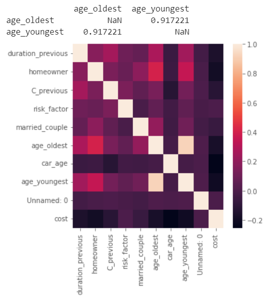There is a high relation between age_youngest and age_oldest which is nearly 0.92, so we can drop one of them.

4. L1-based feature selection: train a Linear models penalized with the L1 norm, of which many estimated coefficients are zero.
5. Tree-based feature selectio: train a Tree-based estimator to compute impurity-based feature importances, which can be used to discard irrelevant features.
6. Sequential Feature Selection: iteratively finds the best new feature to add to the set of selected features.

Train model_region_no_oldest

Refit model_region after dropping these redundant predictor(s); call this model_region_no_oldest.

no_oldest_df = region_df.copy().drop(columns=['age_oldest'])
model_region_no_oldest,X_train, X_test, y_train, y_test  = train_model(no_oldest_df)
print('model_all R2_adj:{},R2:{},aic:{},bic:{}'.format(model_all.rsquared_adj,model_all.rsquared,model_all.aic,model_all.bic))
print('model_sig R2_adj:{},R2:{},aic:{},bic:{}'.format(model_sig.rsquared_adj,model_sig.rsquared,model_sig.aic,model_sig.bic))
print('model_sig_plus R2_adj:{},R2:{},aic:{},bic:{}'.format(model_sig_plus.rsquared_adj,model_sig_plus.rsquared,model_sig_plus.aic,model_sig_plus.bic))
print('model_region R2_adj:{},R2:{},aic:{},bic:{}'.format(model_region.rsquared_adj,model_region.rsquared,model_region.aic,model_region.bic))
print('model_region_no_oldest R2_adj:{},R2:{},aic:{},bic:{}'.format(model_region_no_oldest.rsquared_adj,model_region_no_oldest.rsquared,model_region_no_oldest.aic,model_region_no_oldest.bic))

results:

train mse:1246.680212424389,test mse:1304.1812575671054
model_all R2_adj:0.43278682290809556,R2:0.4359469124696088,aic:123716.65454964116,bic:124236.35709534601
model_sig R2_adj:0.434129203154096,R2:0.43723612396035527,aic:123663.43854360115,bic:124175.71676722451
model_sig_plus R2_adj:0.4984305951183914,R2:0.5172217298672865,aic:122556.63183599956,bic:126008.94160389614
model_region R2_adj:0.4238959955026639,R2:0.4438049590815787,aic:124355.33964859367,bic:127540.3738215563
model_region_no_oldest R2_adj:0.42828875812620626,R2:0.448092078494705,aic:124300.31938605946,bic:127492.77788110361

Diagnose model_region_no_oldest

from statsmodels.compat import lzip

res_df = no_oldest_df.copy()
temp_df = pd.get_dummies(res_df).drop(columns=['cost'])
res_df['cost_pred'] = model_region_no_oldest.predict(temp_df)
res_df['residual'] = res_df['cost_pred'] - res_df['cost']
# print(res_df.columns)
sns.pairplot(res_df,y_vars=['residual'],x_vars=res_df.columns)
plt.show()
plt.figure(figsize=(20,5))
plt.subplot(1,4,1)
plt.hist(res_df['residual'], 
    density=True,     # the histogram integrates to 1 
                      # (so it can be compared to the normal distribution)
    bins=100,         #  draw a histogram with 100 bins of equal width
    label="residuals" # label for legend
    )
# now plot the normal distribution for comparison
xx = np.linspace(res_df['residual'].min(), res_df['residual'].max(), num=1000)
plt.plot(xx, scipy.stats.norm.pdf(xx, loc=0.0, scale=np.sqrt(model_region_no_oldest.scale)),
    label="normal distribution")
outliers = np.abs(res_df['residual'])>4*np.sqrt(model_region_no_oldest.scale)
sns.rugplot(res_df['residual'][outliers],
            color="C5", # otherwise the rugplot has the same color as the histogram
            label="outliers")
plt.legend(loc="upper right")
ax=plt.subplot(1,4,2)
_, (__, ___, r) = scipy.stats.probplot(res_df['residual'], plot=ax, fit=True)
ax=plt.subplot(1,4,3)
sns.residplot(x='cost_pred', y='residual', data=res_df, lowess=True, 
                     scatter_kws={'alpha': 0.5}, 
                     line_kws={'color': 'red', 'lw': 1, 'alpha': 0.8})
plt.subplot(1,4,4)
bins = np.arange(0,50,10)
sqft_bin = np.digitize(res_df['car_age'], bins)
temp_y = res_df['residual'].to_numpy()
sns.scatterplot(x='car_age',y='residual',data=res_df, s=10, alpha=0.3, color="grey")
plt.violinplot([temp_y[sqft_bin == ibin] for ibin in range(1,len(bins)+1)],
               positions=bins,
               widths=5,
               showextrema=True,
               )
plt.show()
name = ['Lagrange multiplier statistic', 'p-value', 'f-value', 'f p-value']
test = sm.stats.het_breuschpagan(model_region_no_oldest.resid, model_region_no_oldest.model.exog)
print(lzip(name, test))

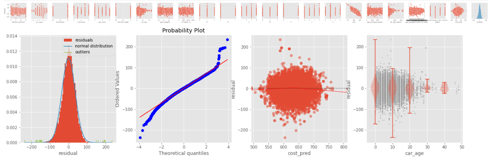
1. The peak of the residuals is higher than the normal distribution
2. Fat tail: both the ends of the Q-Q plot to deviate from the straight line and its center follows a straight line, so there are some large outliers on both sides.
3. Linearity: in the residual plot, the red line which indicates the fit of a locally weighted scatterplot smoothing is almost equal to the dotted horizontal line where the residuals are zero. This is an indication for a linear relationship.
4. Heteroscedasticity: the residuals doesn't spread equally wide with an increase of x, and the Breusch-Pagan Lagrange Multiplier test statistics is also significant(p-value < 0.05), which reject the null hypothesis of homoscedasticity.
5. The violin plots show that the residuals get narrower as car age get larger, which demonstrates heteroscedasticity.

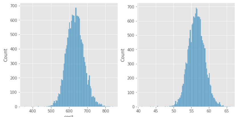
Box-Cox transformation

Find the best Box-Cox transformation of cost used to fit model_region_no_oldest

from scipy.stats import boxcox 

def tran_box_cox(df,col):
    val = df[col]
    if df[col].min() == 0:
        val = val + 1
    transformed_data, best_lambda = boxcox(val) 
    plt.figure(figsize=(10,5))
    plt.subplot(1,2,1)
    sns.histplot(df[col])
    plt.subplot(1,2,2)
    sns.histplot(transformed_data)
    plt.show()
    tran_df = df.copy()
    tran_df[col] = transformed_data
    return tran_df
    
tran_df = tran_box_cox(no_oldest_df,'cost')

Train model_region_no_oldest_box_cox.

model_region_no_oldest_box_cox,X_train, X_test, y_train, y_test  = train_model(tran_df)
print('model_all R2_adj:{},R2:{},aic:{},bic:{}'.format(model_all.rsquared_adj,model_all.rsquared,model_all.aic,model_all.bic))
print('model_sig R2_adj:{},R2:{},aic:{},bic:{}'.format(model_sig.rsquared_adj,model_sig.rsquared,model_sig.aic,model_sig.bic))
print('model_sig_plus R2_adj:{},R2:{},aic:{},bic:{}'.format(model_sig_plus.rsquared_adj,model_sig_plus.rsquared,model_sig_plus.aic,model_sig_plus.bic))
print('model_region R2_adj:{},R2:{},aic:{},bic:{}'.format(model_region.rsquared_adj,model_region.rsquared,model_region.aic,model_region.bic))
print('model_region_no_oldest R2_adj:{},R2:{},aic:{},bic:{}'.format(model_region_no_oldest.rsquared_adj,model_region_no_oldest.rsquared,model_region_no_oldest.aic,model_region_no_oldest.bic))
print('model_region_no_oldest_box_cox R2_adj:{},R2:{},aic:{},bic:{}'.format(model_region_no_oldest_box_cox.rsquared_adj,model_region_no_oldest_box_cox.rsquared,model_region_no_oldest_box_cox.aic,model_region_no_oldest_box_cox.bic))

result:

train mse:2.95842077436262,test mse:3.314232243487904
model_all R2_adj:0.43278682290809556,R2:0.4359469124696088,aic:123716.65454964116,bic:124236.35709534601
model_sig R2_adj:0.434129203154096,R2:0.43723612396035527,aic:123663.43854360115,bic:124175.71676722451
model_sig_plus R2_adj:0.4984305951183914,R2:0.5172217298672865,aic:122556.63183599956,bic:126008.94160389614
model_region R2_adj:0.4238959955026639,R2:0.4438049590815787,aic:124355.33964859367,bic:127540.3738215563
model_region_no_oldest R2_adj:0.42828875812620626,R2:0.448092078494705,aic:124300.31938605946,bic:127492.77788110361
model_region_no_oldest_box_cox R2_adj:0.4327489696162271,R2:0.4524435956206698,aic:49446.489653059136,bic:52646.372470184775

Conclusion

In this, you practiced creating linear models using statsmodels and iteratively trimming the input variables to go from including all the variables in the dataset to using only the most relevant variables. You excluded those variables that were statistically insignificant and removed those that had high correlation. Finally, we performed some feature engineering in an attempt to remove some tail behavior that deviates from the normal distribution to better fit our linear model. In the end, we had a very minimal model that contained variables that other insurance companies use to charge premiums that gave us insight on how we can better serve a niche population.